A water reuse plant gave us an export of its own historian and nothing else. No site visit, no new instruments, no interviews. Twenty-five days of operation: 1,001 tags, 7,172,532 recorded values, 28 June to 23 July.
That export was enough to rank what the plant was losing, and to put an annual figure on each item. This is what the work looked like and what came out of it.
Why a historian export is enough to start
Almost every plant already records far more than anyone reads. A SCADA historian captures every tag on a schedule, forever, and the overwhelming majority of those tags are never looked at unless something breaks. The data is not the constraint. Attention is.
Three properties make that archive useful:
- It is continuous. A lab result describes one moment. A historian describes every moment, which is the only way to see a slope rather than a point.
- It contains pairs. Plants run parallel equipment — twin basins, duty and standby pumps, two membrane trains. Equipment built to do the same job under the same conditions should behave the same way. When it stops, that divergence is a measurement in itself.
- It is already paid for. No capital request, no procurement cycle, no installation window.
The method
For each signal we model what normal looks like for that signal at that plant, rather than against a textbook range. Where the plant publishes its own operating ranges — most do, on the weekly sampling schedule — those become the reference. A finding only counts as a finding if it sits outside the range the plant itself posts.
Then each item is priced, which is the part that decides whether anyone acts:
- Blower power from the isentropic relation, using measured airflow and measured discharge pressure
- Pump power from measured flow and head
- Runtime from historian totaliser deltas
- Everything converted to money using the plant's own tariff
Each line is labelled measured or estimated. Where it is an estimate, the assumptions are written down so the plant's own engineer can check the arithmetic rather than take a vendor's word for it.
What came out
One basin running 3.6x above its own posted range
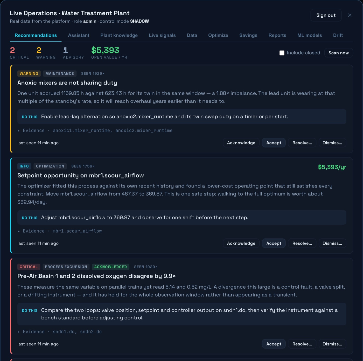
The plant's sampling schedule posts pre-air dissolved oxygen at 0.5–1.5 mg/L. Basin 2 sat right in that band, median 0.49 mg/L. Basin 1 held a median of 5.35 mg/L on every day of the record — roughly eleven times its twin — with its blower command pinned at 99.99%.
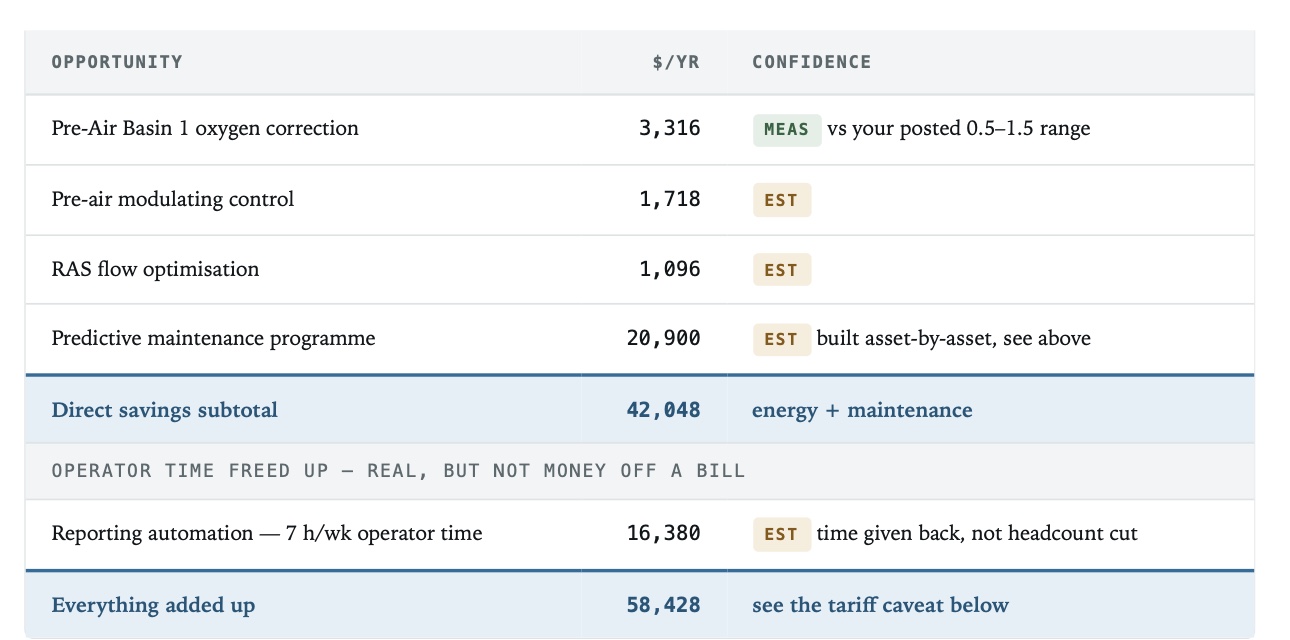
Both basins draw on the same shared air header. That detail is what turns this from a mystery into a maintenance task: if the air supply is common and the outcomes are not, the problem is in the split — a valve or a damper — not in the control strategy. Worth $3,316 a year in blower power, plus the nitrogen-removal risk of carrying that much oxygen into an anoxic zone.
One caveat we put in the report and will repeat here: a fouled DO probe can sit on an offset and still respond to airflow. The reading gets verified against a calibrated handheld before anyone opens a valve.
Membrane scour air above what the flux needed
Airflow tracked the permeate rate almost perfectly — R² of 1.00 — at a ratio well above the manufacturer's specific-scour guidance. Trimming toward the guideline at the measured flux, using the controls already installed, came to $5,391 a year. That was the largest no-capital line on the list.
Pumps starting every twenty-five seconds
Reclaimed water pumps were logging 13 to 28 starts an hour against a manufacturer guideline near six for pumps that size. One asset logged 143 in an hour — a start every twenty-five seconds.
Every start draws locked-rotor current and heats the windings far more than running does. This is a control deadband, not a purchase, and it was quietly writing a bill in motors, starters and contactors: about $3,500 a year.
Sixteen of sixteen reuse totalisers frozen
Every irrigation zone has a volume totaliser. Not one of them changed in twenty-five days.
Until they record, nobody can demonstrate how much recycled water went to beneficial reuse rather than straight to disposal — which is exactly the number a reuse programme is judged on. A configuration fix rather than a purchase, and it unlocks roughly $7,300 a year.
What it added up to
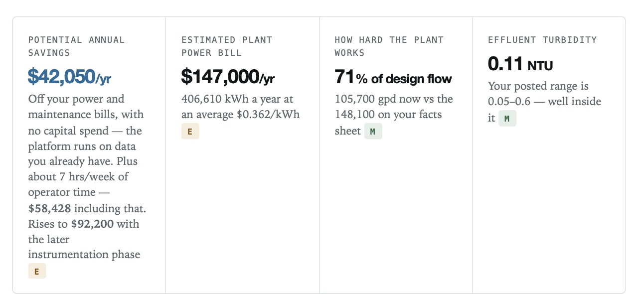
| Direct savings, no capital at all | $42,050 / yr |
| Including ~7 h/week of reporting time returned | $58,428 / yr |
| Fully instrumented, direct | $75,800 / yr |
| Fully instrumented, all in | $92,200 / yr |
Two subtotals are kept deliberately apart: money that comes off a bill, and operator hours given back. The hours are real, but they are not money off a bill, so they never get folded into the first number.
The caveat that matters most
Everything above is priced on a residential time-of-use schedule blending to $0.362/kWh. At 406,610 kWh a year this plant is well past residential scale and would normally sit on a commercial schedule at roughly half that blended rate.
On a commercial tariff, the same physical savings are worth about half what is shown.
The kilowatt-hours are measured either way; only their price is in question, and one utility bill settles it. We put that on the front page of the report rather than in a footnote, because showing the range is worth more than picking the flattering end of it.
What this does not tell you
A twenty-five day window in summer will not capture seasonal variation. Capital figures other than instrumentation are order-of-magnitude and need firming with quotes. And every number here is a ceiling that assumes the recommendation is actually implemented and then maintained — an identified opportunity, not a realised saving.
If your plant keeps a historian, the same exercise is available on your data. It needs an export and nothing else.
Read the full anonymised audit: a membrane-bioreactor water reuse plant.